SerialEM Note: Debug Beam Instability
- Author:
Chen Xu
- Contact:
- Date_Created:
May 31, 2025
- Last_Updated:
May 31, 2025
- Abstract
There are frequent discussions about which software is best for controlling the microscope during cryo-EM operations. One common criticism of SerialEM is that it presents too many details for new users to learn. However, great functionality and flexibility often come with complexity. Personally, I believe this is what makes SerialEM so powerful.
In this note, I share my experience debugging a beam instability issue on the Talos Arctica. I used only two script commands to collect quantitative data—demonstrating how SerialEM can serve as a convenient tool for various types of investigation, thanks to its flexibility.
Background Information
Since the installation of the Talos Arctica, we’ve noticed that the beam appears somewhat unstable. It tends to shift when returning from lower magnifications—even those above the low magnification (LM) range. The beam seems to stabilize after remaining at a single magnification for a longer period. We consulted Thermo Fisher engineers to investigate the issue, but the results were inconclusive.
This instability hasn’t prevented us from routine screening and data collection at good resolution. However, we remain curious whether the issue stems from a problem in the lens system or if we’re simply comparing it—perhaps unfairly—to the Krios. To approach this question more scientifically, we need quantitative data.
Experiment
We set up Low Dose conditions with LD_View at 1250× in uP mode and LD_Record (LD_R) at 36,000× in nP mode. The LD_R beam was adjusted to be small enough so the entire beam could be captured in a single LD_R exposure using the Ceta camera.
We began with the LD_R beam and centered it using the script command CenterBeamFromImage. Then, we cycled between LD_View and LD_Record modes for 50 iterations. During each cycle, we used the script command MeasureBeamPosition to record the X and Y position of the LD_R beam—without re-centering it. This X-Y pair represents the displacement of the beam from the center.
We repeated this process four times and plotted the data to visualize the beam movement.
The script we used is fairly simple, as below:
ScriptName TestBeamStability

echo V=1250 mP R=36000 nP V-F-R-V Similar P1
echo ----------------------------------------

Loop 4

  cycle = 50
    len = $cycle * 2

    NewArray X 0 $cycle
    NewArray Y 0 $cycle
    NewArray XY 0 $len

    #GoToLowDoseArea V
    #Delay 2 s

    R
    CenterBeamFromImage

    Loop $cycle ind
      echo ind = $ind
      ResetClock

      GoToLowDoseArea V
      Delay 0 s
      #GoToLowDoseArea F
      R
      Delay 0 s
      MeasureBeamPosition

      X[$ind] = $repVal1
      Y[$ind] = $repVal2
      even = $ind * 2
      odd = $even - 1
      XY[$odd] = $repVal1
      XY[$even] = $repVal2
      ReportClock
    EndLoop

    Echo X = $X
    Echo Y = $Y
    Echo XY = $XY
    echo ---------------
EndLoop
I also used array function to handle the data more conveniently. In the end or each run, I got some data points as below.
X = -0.28772  7.609619  0.635071  3.970154  3.47998  8.763306  6.890381  8.362732  -3.947632  10.44873  10.689026  4.016235  9.817993  8.887207  3.590088  5.24231  10.75769  7.209595  10.881104  9.042969  5.572937  5.867554  3.767334  4.01123  9.651489  5.485962  10.138306  6.00708  9.137207  8.539063  10.723938  6.897827  2.552856  1.219299  4.884705  -1.502319  2.028076  10.171875  6.290161  8.746338  14.237305  7.865112  5.813354  8.681885  11.348022  7.924805  9.232422  3.668091  5.643311  9.69635
Y = 1.960083  0.892212  -2.176086  1.343628  -2.82959  -5.4104  -0.38324  -0.227539  2.638794  -4.014343  2.027588  2.454956  2.062866  -0.194611  1.811951  -0.455292  -5.424896  -4.145447  -5.28772  1.782349  2.113403  -3.792603  5.762878  1.963867  -1.332825  -0.715271  3.53418  -1.726135  -1.778625  4.091919  -6.234741  -3.225586  3.262817  -0.461731  5.255127  -1.068512  0.04248  0.416626  4.406494  -2.533905  0.589722  2.744873  2.673828  -3.733795  0.639038  0.966675  6.378662  -5.641052  1.754517  4.903931
XY = -0.28772  1.960083  7.609619  0.892212  0.635071  -2.176086  3.970154  1.343628  3.47998  -2.82959  8.763306  -5.4104  6.890381  -0.38324  8.362732  -0.227539  -3.947632  2.638794  10.44873  -4.014343  10.689026  2.027588  4.016235  2.454956  9.817993  2.062866  8.887207  -0.194611  3.590088  1.811951  5.24231  -0.455292  10.75769  -5.424896  7.209595  -4.145447  10.881104  -5.28772  9.042969  1.782349  5.572937  2.113403  5.867554  -3.792603  3.767334  5.762878  4.01123  1.963867  9.651489  -1.332825  5.485962  -0.715271  10.138306  3.53418  6.00708  -1.726135  9.137207  -1.778625  8.539063  4.091919  10.723938  -6.234741  6.897827  -3.225586  2.552856  3.262817  1.219299  -0.461731  4.884705  5.255127  -1.502319  -1.068512  2.028076  0.04248  10.171875  0.416626  6.290161  4.406494  8.746338  -2.533905  14.237305  0.589722  7.865112  2.744873  5.813354  2.673828  8.681885  -3.733795  11.348022  0.639038  7.924805  0.966675  9.232422  6.378662  3.668091  -5.641052  5.643311  1.754517  9.69635  4.903931
With that, I can plot them out to visualize the movement.
Plotting Results
I found an online plotting website which fits my purpose of plotting well. https://www.rapidtables.com/tools/scatter-plot.html. I coped & pasted the XY pairs into webpate and got nice plots. Below are some of the plots from Talos and Glacios.
Fig.1 Beam Movement Talos

Fig.2 Beam Movement Glacios
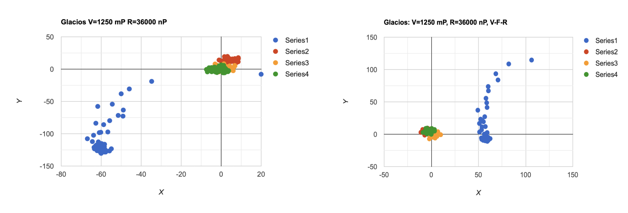
It seems that the beam stabilizes after some time. However, if the cycle is paused for a while—whether in LD_V or LD_R—the beam tends to drift when the cycle resumes. This behavior appears to be related to a dynamic equilibrium, likely caused by thermal changes in the lenses and coils. While the Glacios appears to be marginally more stable, its behavior remains largely comparable to that of the Talos.